Practical Experience in Training Large Language Models: Rejection Sampling
This article is intended for beginners in large language model training. Due to limited experimental resources, some ablation studies remain incomplete, and the conclusions also include subjective reasoning. Friendly discussion in the comments is welcome.
Rejection Sampling
In large language model training, we often hear about SFT and RL, and RL algorithms have become a particular focus over the past two years. Behind these training methods is an idea worth examining: “rejection sampling,” which involves generating candidates and then selecting samples suitable for learning. Today, drawing on my limited practical experience in training large language models, I would like to discuss why rejection sampling matters and how rejecting samples might be more helpful.
If you search directly for “rejection sampling,” you will find many articles explaining it from a statistical perspective; here, we are discussing the practice of generating candidates and filtering data in large language model training, which is not identical to the strictly defined rejection sampling algorithm in statistics. To use an everyday example, Xiaoming is playing basketball for the first time and has no idea how to get the ball into the hoop, so he takes 10 shots in his own way: 6 are terrible and miss everything; 3 are somewhat better and hit the backboard; and on 1 particularly lucky attempt, the ball goes in. He then starts reinforcing the feel of those better shots. In this example, there are 10 samples available for learning, but he selects the 4 better attempts; in other words, he samples 10 times, keeps 4, and rejects 6.
In large language models, rejection sampling is widely used to prepare SFT data [1]. For example, the model can perform multiple rollouts for each task, retaining the trajectory of each attempt, after which a reference answer or a rule-based verifier is used to assign scores, reject low-scoring trajectories, and keep high-scoring ones for SFT.
Beginners may wonder: if a task already has an answer, why not let the model learn the answer directly? There are many reasons:
- First, there may be only an answer, without a solution process or a chain of thought (CoT); learning this way is more like memorizing answers and may offer limited help in developing reasoning ability.
- Second, even when solution steps are available, they may not suit the current model, which may still be unable to reproduce the reasoning independently after learning them. An everyday example comes from doing mathematics in high school: some exercises provided complete, step-by-step solutions, and every step seemed fine when I read through them, yet I found myself unable to solve the problems independently from scratch. This is because a step-by-step solution is a product of thinking and does not necessarily present the thinking process in full. I need to understand how those steps were conceived in order to improve.
One useful approach, therefore, is to let the model try the task itself; if it fails on the first attempt, let it try multiple times, one of which may succeed, and then learn from the complete reasoning process presented in that successful trajectory.
At this point, you may be thinking: does this not resemble reinforcement learning algorithms such as GRPO [2], where the model first makes multiple attempts, then compares which trajectories are better and reinforces the corresponding behavior? Indeed, both SFT after rejection sampling and on-policy RL can use trajectories generated by the model itself and evaluation signals from a verifier. Self-generated trajectories are often closer to the current model’s behavioral distribution, while filtering or reward signals help the model increase the probability of good behavior. However, the training objectives differ: rejection sampling followed by SFT typically imitates only the retained trajectories, whereas RL methods such as GRPO also use relative rewards to adjust the policy, rather than simply discarding low-scoring trajectories.
Another difference between rejection sampling followed by SFT and on-policy RL lies in the frequency of sampling and model updates. The former generally prepares a batch of data first, ranging from hundreds to tens of thousands of examples, and then uses it for training; during training, the data still comes from the old policy model, and this batch may gradually diverge from the current policy as the model is updated [3]. The latter typically alternates more frequently between sampling and updating, keeping the training data closer to the current policy, although recently sampled data may also be reused across multiple updates. For example, if I have 100 exam papers, I can choose to finish all of them at once and then consult the answers to identify and address my weaknesses. Alternatively, I can complete and correct one paper at a time, analyze and learn from it, and then begin the next.
Of course, when relying on successful trajectories or sparse terminal rewards, both rejection sampling and RL need a chance to sample valuable outcomes. If none of 100 attempts succeeds, filtering by correctness may reject every trajectory; RL may also struggle to obtain effective learning signals because the rewards are too sparse. In this situation, these methods are better at turning low-probability successes into high-probability successes, but it is difficult to learn tasks that have almost never been completed successfully through this sampling and feedback alone. For ways to create learning opportunities for such tasks, you can refer to the topic of “curriculum learning,” which I will not discuss further here.
Stepping on Your Own Feet to Ascend (Really?)
Many people may feel that a model can keep growing more capable simply by making multiple attempts itself and retaining the good ones for training; without assistance from other models, the entire system seems to receive no additional information, so is this like “stepping on your own feet to ascend”?
I do not think so, because a crucial component has been overlooked: the verifier. The prerequisite for all of this is that the verifier can evaluate each trajectory against reliable, verifiable criteria and provide rewards with sufficient discriminatory power. There are two key requirements here: verifiability and discriminatory power. If either is missing, effective filtering may become impossible.
As an example of verifiability, suppose we ask a model to make 100 attempts to explore hypotheses about the origin of the universe and then select the better ones for learning; without verifiable evaluation criteria, it is difficult to reliably judge which hypotheses are better, and the selection process lacks a trustworthy learning signal.
As an example of discriminatory power, suppose we ask a model to solve an arithmetic exercise it has already mastered 100 times and then select the better attempts for learning. If most results are correct and scoring considers only whether the final answer is correct, there will be little discriminatory power, and the rejected and retained attempts may be much alike.
Anyone who has worked on benchmarks (such as ResearchClawBench [4]) can probably relate: finding answers or verifiers that are both verifiable and discriminative is very difficult. Often, either all evaluated models can complete the task, leaving no distinction between them, or the models really cannot solve it, only for us to discover that the task itself is unsolvable.
Thus, during rejection sampling, although the verifier does not directly provide a complete solution, it supplies additional information through evaluation, and constructing it also requires substantial knowledge that is difficult to obtain. Rejection sampling is not entirely an emergence of the model’s own capabilities; it can also be viewed as a form of “indirect distillation” of the verifier’s evaluation criteria into the model.
How to Reject Samples
So, how can we reject samples in a way that better trains the model? Suppose I have 100 tasks and let the model attempt each one 10 times, producing 1,000 samples. After scoring, every sample has a score, and the next step is to decide which samples to reject.
First, we can filter the 10 samples for each task. For the same task, we usually learn from a few higher-scoring trajectories and reject low-scoring ones, which is straightforward. But taking this further, do all 100 tasks need to be learned? Some tasks are difficult, with low scores on all 10 attempts, so they seem like candidates for rejection. But if all 10 attempts receive high scores, the task is easy and the model has already mastered it, so it also seems reasonable to reduce such data.
Thinking further, two dimensions jointly influence a sample’s score: task difficulty and model performance. We can use the horizontal axis to represent task difficulty and the vertical axis to represent model performance, with the origin (0, 0) representing typical difficulty and typical performance. All samples are then divided into four quadrants:
- Quadrant I: high task difficulty and good model performance. This is like solving the final, most challenging problem on an exam.
- Quadrant II: low task difficulty and good model performance. This is like correctly answering an easy multiple-choice question on an exam.
- Quadrant III: low task difficulty and poor model performance. This is like getting an easy multiple-choice question wrong on an exam.
- Quadrant IV: high task difficulty and poor model performance. This is like failing to solve the final, most challenging problem on an exam.
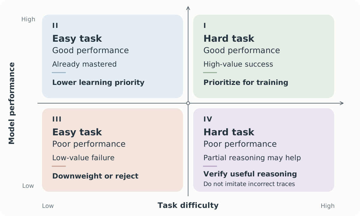
Figure 1: A qualitative division of task difficulty and model performance, with the center representing typical difficulty and typical performance.
Overall, we want to retain samples from Quadrant I for training, because these tasks are difficult and the model performs well, making them worth learning from and reinforcing. At the same time, we want to minimize samples from Quadrant III, where the task is easy but the model underperforms and still gets it wrong. Quadrants II and IV correspond to success on easy tasks and failure on difficult tasks, respectively; these are relatively common situations, and whether to learn from them can be decided case by case.
Some may wonder: why learn from a difficult task when the model gets it wrong? In fact, the model’s trajectory on a difficult task is not necessarily entirely incorrect and may contain valuable reasoning; if these useful parts can be verified and extracted, they may still have learning value, but the entire incorrect trajectory should not be imitated as a correct solution.
Overall, we now have a goal: retain as many samples from Quadrant I as possible and reject samples from Quadrant III.
So, how do we distinguish these samples?
Good model performance is relatively easy to identify, for example when a sample’s score exceeds a certain threshold, such as the 75th percentile. But how should we measure difficulty? The standard deviation of scores across multiple rollouts for each task can, to some extent, reflect the model’s instability on that task, serving as a proxy for difficulty that offers learning value for the current model. Standard deviation is the square root of variance; for the same sets of scores, the two give the same ranking of task variability. Repeated attempts on easy tasks usually produce similar results and a small standard deviation; on some harder tasks, the model sometimes succeeds and sometimes fails, and such tasks may be more worth learning from. Of course, tasks that are too difficult to complete across repeated attempts may also have a small score standard deviation, so it cannot be equated directly with a task’s absolute difficulty.
To examine the relationship between score standard deviation and task difficulty, I created the visualization below. The model under analysis is GLM-5.2, with Opus 4.8 as the comparison baseline. Within this set of tasks, both models may complete the easy ones, while Opus 4.8 may pull ahead of GLM-5.2 on harder ones. The horizontal axis represents the screening threshold: GLM-5.2 first attempts each task 4 times, the standard deviation of the scores is calculated, and tasks are then filtered using different thresholds. For example, x = 0.5 means rejecting tasks with a score standard deviation below 0.5 points. The vertical axis represents the proportion of retained tasks on which the score of Opus 4.8 exceeds the average of GLM-5.2’s 4 attempts by at least a specified margin, with different curves corresponding to different score-gap thresholds. For example, the “gap ≥ 2%” curve represents the proportion of tasks on which Opus 4.8 scores at least 2 points higher; the scores here have been normalized to 0–100, and the “%” in the figure should be understood on that scale.
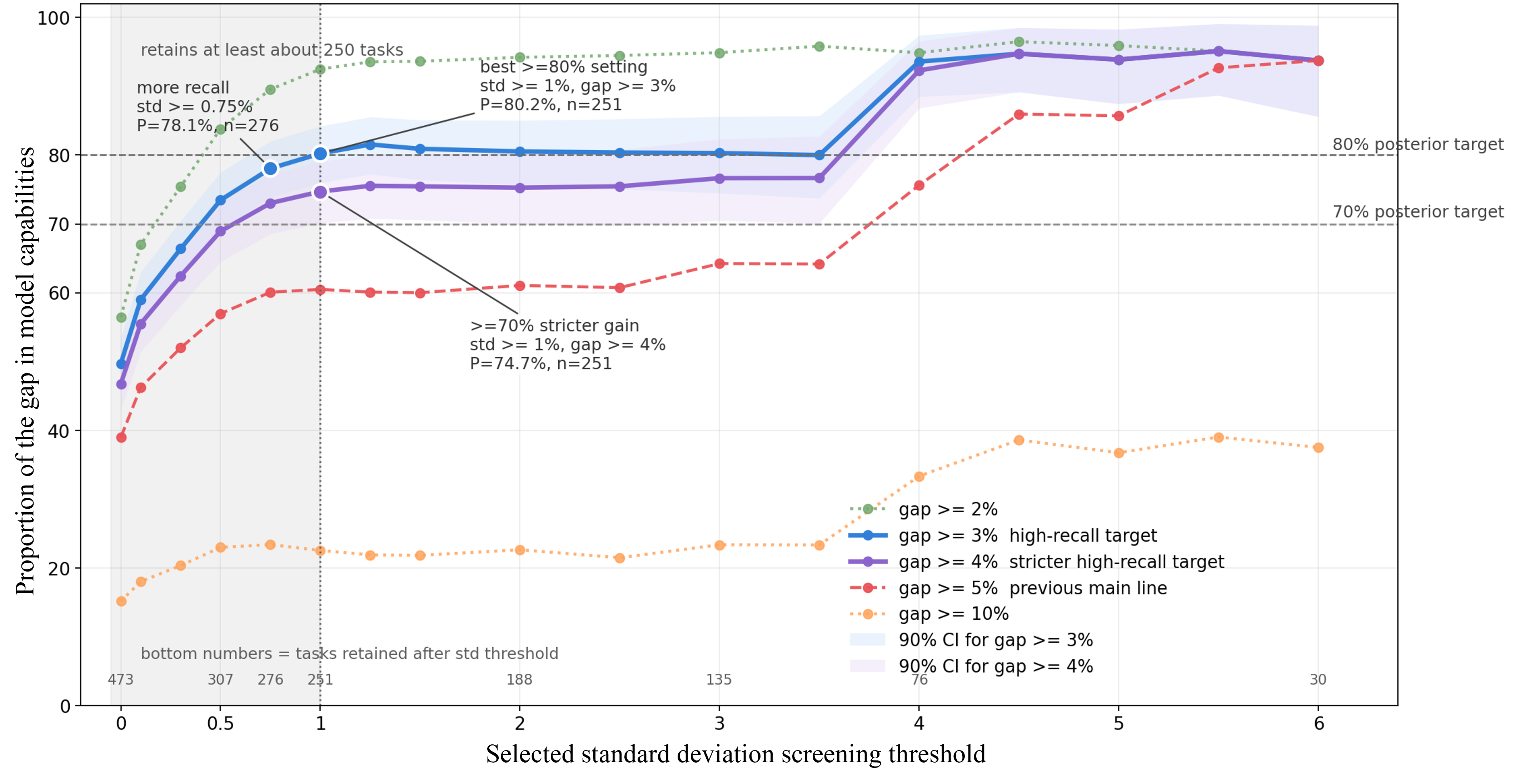
Figure 2: The relationship between the standard deviation threshold, the number of retained tasks, and the model score gap; shaded bands indicate the 90% confidence intervals for the corresponding curves.
The curves show an overall upward trend, although they are not strictly monotonic. In other words, among tasks with a higher score standard deviation, the proportion on which Opus 4.8 exceeds GLM-5.2 by at least a specified margin is generally higher. Of course, an excessively high screening threshold rejects too many tasks, leaving too few training samples available. In this figure, retaining tasks with a standard deviation greater than or equal to 1 point, written as 1% in the figure, offers a reasonable trade-off and corresponds to the highlighted circles with white borders. After rejecting tasks with a standard deviation below 1 point, 251 tasks remain, and on 80.2% of them, Opus 4.8 scores at least 3 points above the average of GLM-5.2’s 4 attempts. This indicates that, in this experiment, the retained tasks better distinguish the two models, and it also supports using score variability as a proxy for difficulty.
Note: This analysis concerns only privately constructed tasks and does not represent the overall capabilities of these two models.
Training Validation
On MLE-bench Lite [5], I compared the following three settings:
- The original Qwen 3.8 27B model.
- Using Qwen 3.8 27B to perform 3 rollouts for each of 2,000 training tasks, retaining the best trajectory for each task and then training on the resulting 2,000 samples, which means selecting samples solely for good model performance.
- First selecting the 600 tasks with the highest score standard deviation from the tasks above, then retaining the best trajectory for each task and training on these 600 samples.
The training results show that, in this experiment, rejection sampling based on model performance improved the model’s performance; after further rejecting tasks with smaller score standard deviations and lower discriminatory power, using only 30% of the data produced even better results. This suggests that task selection based on score variability can help further identify higher-quality, more valuable training data.
Although it is nothing new in AI for a small amount of high-quality data to produce better training results than a large amount of uneven-quality data, I was still surprised when I observed it in my own experiment. The difference in data volume was also substantial: just 30% was enough to outperform the larger dataset.
Table 1: Qwen 3.8 27B results on MLE-bench Lite; Human rank is a normalized metric, with higher values indicating better performance.
| Training setting | Human rank ↑ |
|---|---|
| 1: Original Qwen 3.8 27B (before this SFT) | 0.668 |
| 2: SFT: best trajectory per task (2,000 samples) | 0.693 |
| 3: SFT: best trajectories from the top 600 tasks by score standard deviation | 0.723 |
A Lesson for Life
Life also calls for rejection sampling. If we learn everything, good or bad, without rejecting anything, we may well go astray. If we learn only from good examples but do not filter out overly simple material, we will improve, but perhaps somewhat slowly. If we reject the bad and overly simple material and instead learn from content that is difficult and challenging, we may improve faster.